Basics : Linear Regression
Objective: Given the customer data of a company, whether it should focus on their website or mobile app experience to increase sales.
Source: Udemy | Python for Data Science and Machine Learning Bootcamp
Data used in the below analysis: link
#Import all the libraries for data analysis
import pandas as pd
import numpy as np
import matplotlib.pyplot as plt
import seaborn as sns
#used to view plots within jupyter notebook
%matplotlib inline
sns.set_style("whitegrid") #setting view for plots, optional
customers = pd.read_csv('Ecommerce Customers') #import dataset
customers.head(2) #view dataset
| Address | Avatar | Avg. Session Length | Time on App | Time on Website | Length of Membership | Yearly Amount Spent | ||
|---|---|---|---|---|---|---|---|---|
| 0 | mstephenson@fernandez.com | 835 Frank Tunnel\nWrightmouth, MI 82180-9605 | Violet | 34.497268 | 12.655651 | 39.577668 | 4.082621 | 587.951054 |
| 1 | hduke@hotmail.com | 4547 Archer Common\nDiazchester, CA 06566-8576 | DarkGreen | 31.926272 | 11.109461 | 37.268959 | 2.664034 | 392.204933 |
#view some informormation of the dataset
customers.describe()
| Avg. Session Length | Time on App | Time on Website | Length of Membership | Yearly Amount Spent | |
|---|---|---|---|---|---|
| count | 500.000000 | 500.000000 | 500.000000 | 500.000000 | 500.000000 |
| mean | 33.053194 | 12.052488 | 37.060445 | 3.533462 | 499.314038 |
| std | 0.992563 | 0.994216 | 1.010489 | 0.999278 | 79.314782 |
| min | 29.532429 | 8.508152 | 33.913847 | 0.269901 | 256.670582 |
| 25% | 32.341822 | 11.388153 | 36.349257 | 2.930450 | 445.038277 |
| 50% | 33.082008 | 11.983231 | 37.069367 | 3.533975 | 498.887875 |
| 75% | 33.711985 | 12.753850 | 37.716432 | 4.126502 | 549.313828 |
| max | 36.139662 | 15.126994 | 40.005182 | 6.922689 | 765.518462 |
customers.info()
<class 'pandas.core.frame.DataFrame'>
RangeIndex: 500 entries, 0 to 499
Data columns (total 8 columns):
 #   Column                Non-Null Count  Dtype
---  ------                --------------  -----
 0   Email                 500 non-null    object
 1   Address               500 non-null    object
 2   Avatar                500 non-null    object
 3   Avg. Session Length   500 non-null    float64
 4   Time on App           500 non-null    float64
 5   Time on Website       500 non-null    float64
 6   Length of Membership  500 non-null    float64
 7   Yearly Amount Spent   500 non-null    float64
dtypes: float64(5), object(3)
memory usage: 31.4+ KB
#View numerics data in the dataset and the relationship with other columns
sns.pairplot(data=customers)
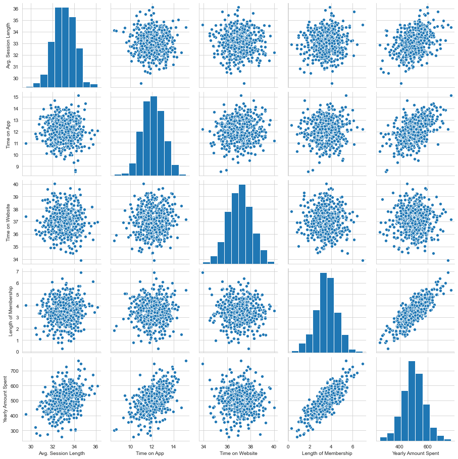
It seems Lenth of Membership is most correlated with Yearly Amount Spent
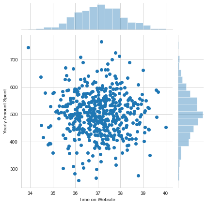
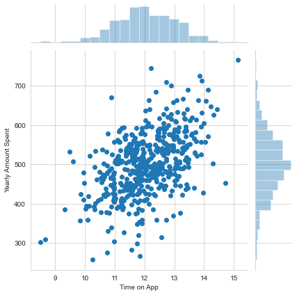
#Playing aorund with the data to check for more correlations
sns.jointplot(x='Time on Website',y='Yearly Amount Spent',data=customers)
sns.jointplot(x='Time on App',y='Yearly Amount Spent',data=customers)
sns.jointplot(x='Time on App',y='Length of Membership',data=customers,kind='hex')
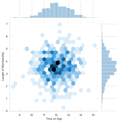
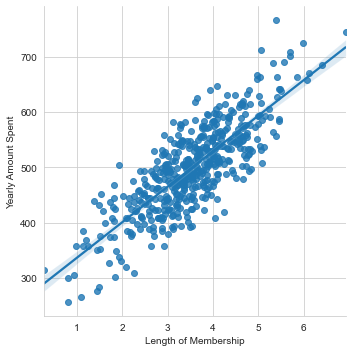
#Can see the correlation clearly here
sns.lmplot(x='Length of Membership',y='Yearly Amount Spent', data = customers)
Now we start training the model to predict Yearly Amount spent based on given information
#view column names in the dataset
customers.columns
Index(['Email', 'Address', 'Avatar', 'Avg. Session Length', 'Time on App',
       'Time on Website', 'Length of Membership', 'Yearly Amount Spent'],
      dtype='object')
#divide data into X and y DataFrames
X = customers[['Avg. Session Length', 'Time on App',
       'Time on Website', 'Length of Membership']]
y = customers['Yearly Amount Spent']
#Split the X and y into Training and Test
from sklearn.model_selection import train_test_split
X_train,X_test, y_train,y_test =train_test_split(X, y, test_size=0.3, random_state=101)
#import Linear Regression model from Sci-kit Learn
from sklearn.linear_model import LinearRegression
lm = LinearRegression()
lm.fit(X_train,y_train)
LinearRegression()
#view coefficients, or amount of correlation among Yearly Amount spent and other data provided
lm.coef_
array([25.98154972, 38.59015875, 0.19040528, 61.27909654])
#predict the values on the test data
predictions = lm.predict(X_test)
#plot the result alongwith the actual data
plt.scatter(y_test,predictions)
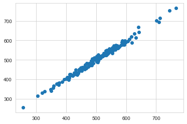
Model rendered seems like a good fit
#import metrics to evaluate model performance
from sklearn import metrics
print('MAE:', metrics.mean_absolute_error(y_test, predictions))
print('MSE:', metrics.mean_squared_error(y_test, predictions))
print('RMSE:', np.sqrt(metrics.mean_squared_error(y_test, predictions)))
MAE: 7.228148653430839
MSE: 79.81305165097469
RMSE: 8.933815066978648
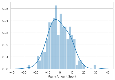
#plot the residual amount to check model performance
sns.distplot(y_test-predictions,bins=30)
Check the correlation with coefficients seen before
Coeff = pd.DataFrame(lm.coef_,X.columns,columns=['Coefficients'])
Coeff
| Coefficients | |
|---|---|
| Avg. Session Length | 25.981550 |
| Time on App | 38.590159 |
| Time on Website | 0.190405 |
| Length of Membership | 61.279097 |
The above data signify that 1 change in Avg. Session Length will lead to 25.98 change in Yearly Amount Spent.
Similarly, for Time on App, Time on Website and Length of Membership
As predicted before, the most impact if from Length of Membership
