Basics : Support Vector Machines
Objective: Apply SVM (Support Vector Machines) to the popular Iris dataset and classify the flowers on the basis of their features.
Source: Udemy | Python for Data Science and Machine Learning Bootcamp
#importing libraries to be used
import numpy as np
import pandas as pd
import matplotlib.pyplot as plt
import seaborn as sns
#view plots in jupyter notebook
%matplotlib inline
sns.set_style('whitegrid') #setting style for plots, optional
#importing data from the seaborn datasets
iris = sns.load_dataset('iris')
#check data info
iris
| sepal_length | sepal_width | petal_length | petal_width | species | |
|---|---|---|---|---|---|
| 0 | 5.1 | 3.5 | 1.4 | 0.2 | setosa |
| 1 | 4.9 | 3.0 | 1.4 | 0.2 | setosa |
| 2 | 4.7 | 3.2 | 1.3 | 0.2 | setosa |
| 3 | 4.6 | 3.1 | 1.5 | 0.2 | setosa |
| 4 | 5.0 | 3.6 | 1.4 | 0.2 | setosa |
| ... | ... | ... | ... | ... | ... |
| 145 | 6.7 | 3.0 | 5.2 | 2.3 | virginica |
| 146 | 6.3 | 2.5 | 5.0 | 1.9 | virginica |
| 147 | 6.5 | 3.0 | 5.2 | 2.0 | virginica |
| 148 | 6.2 | 3.4 | 5.4 | 2.3 | virginica |
| 149 | 5.9 | 3.0 | 5.1 | 1.8 | virginica |
150 rows × 5 columns
#visualize/explore dataset
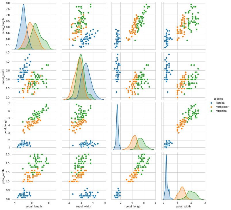
sns.pairplot(data=iris,hue='species')

The species ‘Setosa’ seems to be the most separable
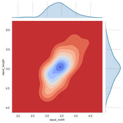
sns.jointplot(x='sepal_width',y='sepal_length',data=iris[iris['species']=='setosa'],kind='kde',cmap='coolwarm_r')

Split data into Train and test datasets and train model
from sklearn.model_selection import train_test_split
X_train, X_test, y_train, y_test = train_test_split(iris.drop('species',axis=1),iris['species'],test_size=0.3, random_state=101)
from sklearn.svm import SVC
model_svc = SVC()
model_svc.fit(X_train,y_train)
SVC()
predictions = model_svc.predict(X_test)
from sklearn.metrics import classification_report, confusion_matrix
print(confusion_matrix(y_test,predictions))
[[13  0  0]
 [ 0 19  1]
 [ 0  0 12]]
print(classification_report(y_test,predictions))
              precision    recall  f1-score   support

      setosa       1.00      1.00      1.00        13
  versicolor       1.00      0.95      0.97        20
   virginica       0.92      1.00      0.96        12

    accuracy                           0.98        45
   macro avg       0.97      0.98      0.98        45
weighted avg       0.98      0.98      0.98        45
The model is already a good fit with an accuracy of 98%. But usually, we might not get such results with default parameters in SVM and we need to do cross validations to get the best parameters to run our model. We can do this with GridSearch.
Gridsearch Practise
from sklearn.model_selection import GridSearchCV
#Creating a dictionary to sepcify values to do cross validation on
param_grid = {'C': [0.1,1, 10, 100, 1000], 'gamma': [1,0.1,0.01,0.001,0.0001]}
grid = GridSearchCV(SVC(),param_grid,refit=True,verbose=3)
grid.fit(X_train,y_train)
Fitting 5 folds for each of 25 candidates, totalling 125 fits
[CV] C=0.1, gamma=1 ..................................................
[CV] ...................... C=0.1, gamma=1, score=0.905, total=   0.0s
[CV] C=0.1, gamma=1 ..................................................
[CV] ...................... C=0.1, gamma=1, score=1.000, total=   0.0s
[CV] C=0.1, gamma=1 ..................................................
[CV] ...................... C=0.1, gamma=1, score=0.905, total=   0.0s
[CV] C=0.1, gamma=1 ..................................................
[CV] ...................... C=0.1, gamma=1, score=0.905, total=   0.0s
[CV] C=0.1, gamma=1 ..................................................
.
.
.
[CV] C=1, gamma=0.001 ................................................


[Parallel(n_jobs=1)]: Using backend SequentialBackend with 1 concurrent workers.
[Parallel(n_jobs=1)]: Done   1 out of   1 | elapsed:    0.0s remaining:    0.0s
[Parallel(n_jobs=1)]: Done   2 out of   2 | elapsed:    0.0s remaining:    0.0s


[CV] .................... C=1, gamma=0.001, score=0.714, total=   0.0s
[CV] C=1, gamma=0.001 ................................................
[CV] .................... C=1, gamma=0.001, score=0.714, total=   0.0s
[CV] C=1, gamma=0.001 ................................................
[CV] .................... C=1, gamma=0.001, score=0.714, total=   0.0s
[CV] C=1, gamma=0.0001 ...............................................
[CV] ................... C=1, gamma=0.0001, score=0.333, total=   0.0s
.
.
.
[CV] ................ C=1000, gamma=0.0001, score=1.000, total=   0.0s


[Parallel(n_jobs=1)]: Done 125 out of 125 | elapsed:    0.6s finished


GridSearchCV(estimator=SVC(),
             param_grid={'C': [0.1, 1, 10, 100, 1000],
                         'gamma': [1, 0.1, 0.01, 0.001, 0.0001]},
             verbose=3)
n_predictions = grid.predict(X_test)
print(confusion_matrix(y_test,n_predictions))
[[13  0  0]
 [ 0 19  1]
 [ 0  0 12]]
print(classification_report(y_test,n_predictions))
              precision    recall  f1-score   support

      setosa       1.00      1.00      1.00        13
  versicolor       1.00      0.95      0.97        20
   virginica       0.92      1.00      0.96        12

    accuracy                           0.98        45
   macro avg       0.97      0.98      0.98        45
weighted avg       0.98      0.98      0.98        45
